Legendre Polynomials

Legendre polynomials, $ P_n(x) $, are a sequence of orthogonal polynomials that are solutions to the Legendre differential equation:

\[(1 - x^2) \frac{d^2 P_n(x)}{dx^2} - 2x \frac{d P_n(x)}{dx} + n(n + 1) P_n(x) = 0\]

where $ n $ is a non-negative integer, and $ P_n(x) $ represents the nth Legendre polynomial. These polynomials are used extensively in physics and engineering, particularly in solving problems that exhibit spherical symmetry, such as potential theory and quantum mechanics.

Derivation of Legendre Polynomials

Legendre polynomials can be derived using several methods, such as series solutions or recurrence relations. Below are the two main methods of obtaining these polynomials:

1. Series Solution Method

To derive Legendre polynomials, we begin by solving the Legendre differential equation using a power series expansion. The general solution can be written as a power series around $ x = 0 $:

\[P_n(x) = \sum_{k=0}^{\infty} a_k x^k\]

Substituting this series into the Legendre differential equation and solving for the coefficients ($ a_k $ results in a series that converges for $ |x| \leq 1 $. This method leads to the explicit expression for Legendre polynomials for low values of $ n $.

For example, for the first few polynomials:

• $ P_0(x) = 1 $

• $ P_1(x) = x $

• $ P_2(x) = \frac{1}{2} (3x^2 - 1) $

• $ P_3(x) = \frac{1}{2} (5x^3 - 3x) $

2. Recurrence Relation Method

Another method for obtaining Legendre polynomials is through a recurrence relation. Starting with known values for $ P_0(x) $ and $ P_1(x) $, the following recurrence relation can be used to compute higher-order polynomials:

\[(n+1) P_{n+1}(x) = (2n+1) x P_n(x) - n P_{n-1}(x)\]

with the initial conditions:

\[P_0(x) = 1, \quad P_1(x) = x\]

Using this recurrence, we can generate higher-order Legendre polynomials:

• For $ n = 2 $, $ P_2(x) = \frac{1}{2} (3x^2 - 1) $

• For $ n = 3 $, $ P_3(x) = \frac{1}{2} (5x^3 - 3x) $

• For $ n = 4 $, $ P_4(x) = \frac{1}{8} (35x^4 - 30x^2 + 3) $

This recurrence relation provides a straightforward method to generate Legendre polynomials of any degree.

Alternate Recurrence Relation

Another form of the recurrence relation for Legendre polynomials is:

\[P_l(x) = \frac{(2l - 1) x P_{l-1}(x) - (l - 1) P_{l-2}(x)}{l}\]

Derivation of This Recurrence Relation

This recurrence relation can be derived directly from the Legendre differential equation. To understand its origin, consider the standard recurrence relation for Legendre polynomials:

\[(n + 1) P_{n+1}(x) = (2n + 1) x P_n(x) - n P_{n-1}(x)\]

By changing the index from ( n ) to ( l ), we obtain:

\[l P_l(x) = (2l - 1) x P_{l-1}(x) - (l - 1) P_{l-2}(x)\]

Dividing both sides of the equation by $ (l) $, we get:

\[P_l(x) = \frac{(2l - 1) x P_{l-1}(x) - (l - 1) P_{l-2}(x)}{l}\]

This is the recurrence relation you provided. It expresses $ P_l(x) $ in terms of the two previous polynomials, $ P_{l-1}(x) $ and $P_{l-2}(x) $, and is helpful for computing higher-order Legendre polynomials when the lower-order ones are known.

Properties of Legendre Polynomials

1. Orthogonality: The Legendre polynomials are orthogonal with respect to the weight function $ w(x) = 1 $ over the interval $ [-1, 1] $. Specifically, for any two different Legendre polynomials $ P_n(x) $ and $ P_m(x) $, the following orthogonality condition holds:

   \[\int_{-1}^{1} P_n(x) P_m(x) \, dx = 0 \quad \text{for} \quad n \neq m\]

   For $ n = m $, the integral is given by:

   \[\int_{-1}^{1} P_n(x)^2 \, dx = \frac{2}{2n + 1}\]

2. Recurrence Relations: As mentioned, Legendre polynomials satisfy a recurrence relation, which is useful for calculating higher-degree polynomials from lower-degree ones.

3. Symmetry: Legendre polynomials exhibit symmetry properties. Specifically, $ P_n(-x) = (-1)^n P_n(x) $, meaning that they are either even or odd functions, depending on the degree $ n $.

4. Normalizability: The Legendre polynomials can be normalized so that they are orthonormal, i.e., the integral of their square is 1. This is done by dividing each polynomial by $ \sqrt{\frac{2}{2n+1}} $.

Applications of Legendre Polynomials

Legendre polynomials are widely used in various fields of physics and mathematics. Some of their main applications include:

1. Potential Theory: In solving Laplace’s equation in spherical coordinates, Legendre polynomials are used to expand the solution in terms of spherical harmonics.

2. Quantum Mechanics: Legendre polynomials appear in the solutions of the Schrödinger equation for spherically symmetric potentials, such as in the hydrogen atom.

3. Numerical Methods: Legendre polynomials are used in Gaussian quadrature for numerical integration, where the roots of the Legendre polynomials serve as optimal sampling points.

4. Electromagnetic Theory: In electrostatics and electromagnetics, Legendre polynomials are used in the expansion of the electric potential and field in spherical coordinates.

In conclusion, Legendre polynomials are essential mathematical tools with significant applications in physics and engineering. They are obtained through either a power series solution to their defining differential equation or using recurrence relations. Their orthogonality and other properties make them invaluable for expanding functions and solving physical problems in spherical geometries.

import numpy as np
import matplotlib.pyplot as plt
from scipy.special import legendre

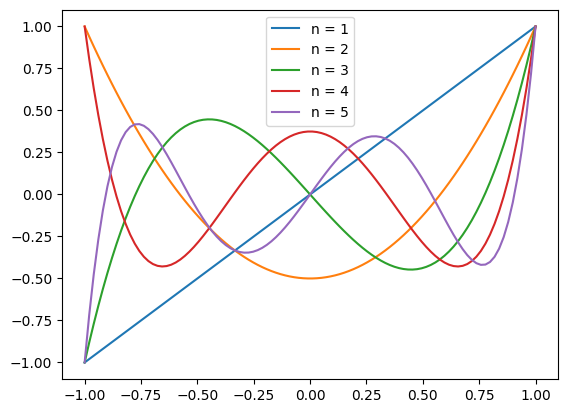
x = np.linspace(-1, 1, 100)

for n in range(1, 6, 1):
    plt.plot(x, legendre(n)(x), label = f"n = {n}")
plt.legend()
plt.show()

from scipy.integrate import quad

def inner_product(m, n):

    P_m = legendre(m)
    P_n = legendre(n)

    integrand = lambda x: P_m(x) * P_n(x)
    result = quad(integrand, -1, 1)[0]

    return result

for m in range(0, 5):
    for n in range(0, 5):
        val = inner_product(m, n)
        if m == n:
            val_expect = 2/(2 * n + 1)
            print(f"P_{m}P_{n} = {val} {val_expect}")

P_0P_0 = 2.0 2.0
P_1P_1 = 0.6666666666666666 0.6666666666666666
P_2P_2 = 0.4 0.4
P_3P_3 = 0.28571428571428575 0.2857142857142857
P_4P_4 = 0.22222222222222224 0.2222222222222222

import numpy as np
from scipy.integrate import quad
from scipy.special import legendre

# Function to verify normalization condition of Legendre polynomials
def verify_normalization(n):
    # Get the Legendre polynomial of degree n using scipy's legendre function
    Pn = legendre(n)

    # Define the integrand (P_n(x))^2
    def integrand(x):
        return Pn(x)**2

    # Perform the numerical integration over the interval [-1, 1]
    result, _ = quad(integrand, -1, 1)

    # Expected normalization constant for Legendre polynomial of degree n
    expected_normalization = 2 / (2 * n + 1)

    print(f"Computed integral for P_{n}(x)^2 over [-1, 1]: {result}")
    print(f"Expected normalization value: {expected_normalization}")

    # Check if the computed result is close to the expected normalization
    if np.isclose(result, expected_normalization, atol=1e-6):
        print(f"P_{n}(x) is correctly normalized!")
    else:
        print(f"P_{n}(x) is NOT correctly normalized!")

# Test for a specific degree n
n = 3  # Example for degree 3
verify_normalization(n)

Computed integral for P_3(x)^2 over [-1, 1]: 0.28571428571428575
Expected normalization value: 0.2857142857142857
P_3(x) is correctly normalized!