Verification of Dirac Delta Function Properties using Gaussian and Rectangular Functions

Introduction

The Dirac Delta function, denoted as \(\delta(x)\), is a generalized function used in mathematical physics and engineering. It is not a conventional function but rather a distribution that models an idealized point source or impulse. The delta function satisfies the sifting property:

\[\int_{-\infty}^{\infty} \delta(x-a) f(x) dx = f(a)\]

for any continuous function \(f(x)\).

To understand the delta function rigorously, we can approximate it using a sequence of well-defined functions. Two common representations are:

1. Gaussian function sequence

2. Rectangular function sequence

We will verify the defining properties of the Dirac Delta function using these representations.

Gaussian Function Representation

A sequence of Gaussian functions that approximates the delta function is given by:

\[\delta_\epsilon(x) = \frac{1}{\sqrt{\pi \epsilon}} e^{-x^2/\epsilon}\]

where \(\epsilon\) is a small positive parameter. As \(\epsilon \to 0\), \(\delta_\epsilon(x)\) becomes increasingly peaked at \(x=0\).

Property 1: Normalization

We verify:

\[\int_{-\infty}^{\infty} \delta_\epsilon(x) dx = 1\]

Calculation:

\[\int_{-\infty}^{\infty} \frac{1}{\sqrt{\pi \epsilon}} e^{-x^2/\epsilon} dx\]

Using the standard Gaussian integral formula:

\[\int_{-\infty}^{\infty} e^{-u^2} du = \sqrt{\pi}\]

we substitute \(u = x/\sqrt{\epsilon}\), giving \(du = dx/\sqrt{\epsilon}\). Then:

\[\int_{-\infty}^{\infty} \frac{1}{\sqrt{\pi \epsilon}} e^{-x^2/\epsilon} dx = \frac{1}{\sqrt{\pi \epsilon}} \cdot \sqrt{\pi \epsilon} = 1\]

Thus, the normalization property holds.

Property 2: Sifting Property

We verify:

\[\int_{-\infty}^{\infty} f(x) \delta_\epsilon(x) dx \approx f(0)\]

Using Taylor expansion at \(x=0\):

\[f(x) \approx f(0) + x f'(0) + O(x^2)\]

Multiplying by \(\delta_\epsilon(x)\) and integrating:

\[\int_{-\infty}^{\infty} f(x) \delta_\epsilon(x) dx = f(0) \int_{-\infty}^{\infty} \delta_\epsilon(x) dx + f'(0) \int_{-\infty}^{\infty} x \delta_\epsilon(x) dx + O(\epsilon)\]

Since \(\int x \delta_\epsilon(x) dx = 0\) by symmetry, we get:

\[\int_{-\infty}^{\infty} f(x) \delta_\epsilon(x) dx = f(0)\]

Thus, the sifting property holds.

Rectangular Function Representation

A sequence of rectangular functions that approximates the delta function is:

\[\begin{split}\delta_\epsilon(x) = \begin{cases} \frac{1}{2\epsilon}, & \text{if } -\epsilon \leq x \leq \epsilon \\ 0, & \text{otherwise} \end{cases}\end{split}\]

Property 1: Normalization

\[\int_{-\infty}^{\infty} \delta_\epsilon(x) dx = \int_{-\epsilon}^{\epsilon} \frac{1}{2\epsilon} dx\]

\[= \frac{1}{2\epsilon} (2\epsilon) = 1\]

Thus, normalization holds.

Property 2: Sifting Property

\[\int_{-\infty}^{\infty} f(x) \delta_\epsilon(x) dx = \int_{-\epsilon}^{\epsilon} f(x) \frac{1}{2\epsilon} dx\]

For small \(\epsilon\), we approximate \(f(x) \approx f(0)\), so:

\[\int_{-\epsilon}^{\epsilon} f(0) \frac{1}{2\epsilon} dx = f(0) \cdot \frac{1}{2\epsilon} \cdot (2\epsilon) = f(0)\]

Thus, the sifting property holds.

Conclusion

Both Gaussian and rectangular function sequences satisfy the normalization and sifting properties, confirming that they are valid representations of the Dirac Delta function. As \(\epsilon \to 0\), these functions increasingly resemble an ideal delta function centered at \(x=0\).

Bibliography

1. Dirac, P. A. M. The Principles of Quantum Mechanics, Oxford University Press, 1930.

2. Arfken, G. B., & Weber, H. J. Mathematical Methods for Physicists, Academic Press, 2005.

3. Bracewell, R. N. The Fourier Transform and Its Applications, McGraw-Hill, 1999.

4. Strichartz, R. S. A Guide to Distribution Theory and Fourier Transforms, World Scientific, 2003.

5. Lighthill, M. J. An Introduction to Fourier Analysis and Generalised Functions, Cambridge University Press, 1958.

Algorithm

1. Define Input Parameters:

   • Small parameter \(\epsilon\)

   • Large interval \(L\)

   • Test function \(f(x)\)

2. Verify Normalization:

   \[I = \int_{-L}^{L} \delta_\epsilon(x) dx\]

   • Compute for both Gaussian and rectangular functions.

   • Compare with expected value \(1\).

3. Verify Sifting Property:

   \[J = \int_{-L}^{L} f(x) \delta_\epsilon(x) dx\]

   • Compute for both Gaussian and rectangular functions.

   • Compare with expected value \(f(0)\).

4. Repeat for Different :math:`epsilon`:

   • Reduce \(\epsilon\) and observe convergence.

---

Python Implementation

The following Python code numerically verifies these properties.

import numpy as np
import scipy.integrate as spi
import matplotlib.pyplot as plt

# Define Gaussian Delta Approximation
def gaussian_delta(x, epsilon):
    return (1 / np.sqrt(np.pi * epsilon)) * np.exp(-x**2 / epsilon)

# Define Rectangular Delta Approximation
def rectangular_delta(x, epsilon):
    return np.where(np.abs(x) <= epsilon, 1 / (2 * epsilon), 0)

# Define Test Function
def test_function(x):
    return np.exp(-x)  # Example function

# Parameters
epsilon_values = [0.1, 0.01, 0.001]  # Decreasing ε
L = 5  # Integration limit

# Perform integration and verification
for epsilon in epsilon_values:
    # Normalization
    norm_gaussian, _ = spi.quad(lambda x: gaussian_delta(x, epsilon), -L, L, limit = 100)
    norm_rectangular, _ = spi.quad(lambda x: rectangular_delta(x, epsilon), -L, L, limit = 100)

    # Sifting property
    sift_gaussian, _ = spi.quad(lambda x: test_function(x) * gaussian_delta(x, epsilon), -L, L, limit = 100)
    sift_rectangular, _ = spi.quad(lambda x: test_function(x) * rectangular_delta(x, epsilon), -L, L, limit = 100)

    print(f"\nFor ε = {epsilon}:")
    print(f"Normalization - Gaussian: {norm_gaussian:.5f}, Rectangular: {norm_rectangular:.5f}")
    print(f"Sifting Property - Gaussian: {sift_gaussian:.5f}, Expected: {test_function(0):.5f}")
    print(f"Sifting Property - Rectangular: {sift_rectangular:.5f}, Expected: {test_function(0):.5f}")

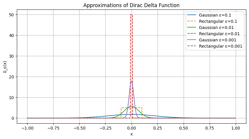
# Plot the approximations for visualization
x_vals = np.linspace(-1, 1, 1000)

plt.figure(figsize=(10, 5))
for epsilon in epsilon_values:
    plt.plot(x_vals, gaussian_delta(x_vals, epsilon), label=f"Gaussian ε={epsilon}")
    plt.plot(x_vals, rectangular_delta(x_vals, epsilon), '--', label=f"Rectangular ε={epsilon}")

plt.xlabel("x")
plt.ylabel("δ_ε(x)")
plt.title("Approximations of Dirac Delta Function")
plt.legend()
plt.grid()
plt.show()

For ε = 0.1:
Normalization - Gaussian: 1.00000, Rectangular: 1.00000
Sifting Property - Gaussian: 1.02532, Expected: 1.00000
Sifting Property - Rectangular: 1.00167, Expected: 1.00000

For ε = 0.01:
Normalization - Gaussian: 1.00000, Rectangular: 0.00000
Sifting Property - Gaussian: 1.00250, Expected: 1.00000
Sifting Property - Rectangular: 0.00000, Expected: 1.00000

For ε = 0.001:
Normalization - Gaussian: 1.00000, Rectangular: 0.00000
Sifting Property - Gaussian: 1.00025, Expected: 1.00000
Sifting Property - Rectangular: 0.00000, Expected: 1.00000