Fourier Series Analysis - Saw Tooth Wave

A sawtooth wave is a periodic function that increases linearly and then drops sharply. It can be expressed using a Fourier series as: \begin{equation} f(x) = \sum_{n=1}^{\infty}\frac{(-1)^{(n+1)}}{n}\sin nx \end{equation}

Algorithm: Fourier Series for a Sawtooth Wave

This algorithm computes and visualizes the Fourier series approximation of a sawtooth wave, which increases linearly and drops sharply at the end of each period.

---

Step 1: Import Required Libraries

• Import numpy for array and mathematical operations.

• Import matplotlib.pyplot for plotting the wave.

---

Step 2: Define Constants

• Define pi as the mathematical constant π using NumPy.

---

Step 3: Loop Through Harmonic Terms

• Loop through odd values of m from 3 to 7 (exclusive upper bound 9, step 2).

  • This determines the number of Fourier terms (harmonics) used in the approximation.

---

Step 4: Generate x and n Values

• xrange: 100 values linearly spaced between -π and π.

• n: Array of integers from 1 to m-1, reshaped as a column vector for broadcasting.

---

Step 5: Compute Fourier Series Sum

• Apply the formula:

  \[f(x) = \sum_{n=1}^{m} \frac{(-1)^{n+1}}{n} \sin(nx)\]

• Use NumPy to compute the sum:

  • Calculate ((-1)^(n+1)) * sin(n * x) / n and sum across harmonics.

  • Store the result in fsum.

---

Step 6: Plot the Result

• Plot fsum against xrange for each value of m.

• Label each curve accordingly.

---

Step 7: Customize Plot

• Set labels for the x and y axes.

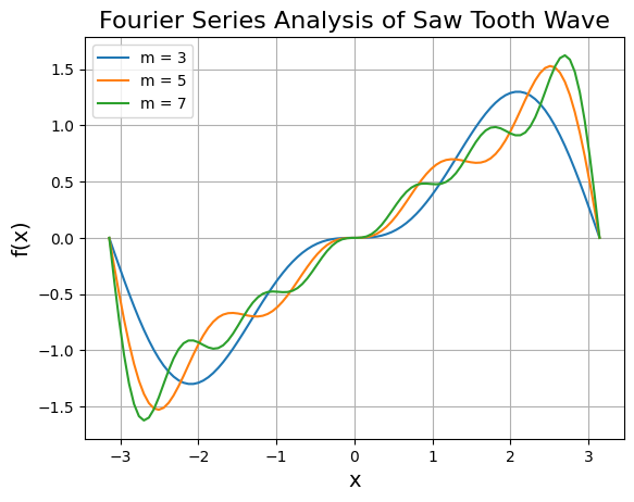
• Add a title: “Fourier Series Analysis of Saw Tooth Wave”

• Add a legend and grid for visual clarity.

---

Step 8: Display the Plot

• Use plt.show() to render the final visualization.

---

Output:

• Multiple curves representing the sawtooth wave using increasing numbers of harmonics (Fourier terms).

import numpy as np
import matplotlib.pyplot as plt

pi = np.pi

for m in range(3, 9, 2):
    xrange = np.linspace(-pi, pi, 100);xrange
    n = np.arange(1, m)[:, np.newaxis]
    fsum = np.sum(((-1)**(n+1)) * np.sin(n * xrange) / n, axis=0)
    plt.plot(xrange, fsum, label = f"m = {m}")
plt.xlabel("x", fontsize =14)
plt.ylabel("f(x)", fontsize =14)
plt.title("Fourier Series Analysis of Saw Tooth Wave", fontsize = 16)
plt.legend()
plt.grid()
plt.show()