Fourier Series Analysis - Square Wave

Fourier series for a square wave function:

\[f(x) = \frac{4k}{\pi}\sum_{n \to \text{odd}}\frac{1}{n}\sin nx\]

Algorithm: Fourier Series for a Square Wave

This algorithm visualizes the Fourier series approximation of a square wave function using Python.

---

Step 1: Import Libraries

• Import numpy for numerical operations.

• Import matplotlib.pyplot for plotting.

---

Step 2: Initialize Constants

• Set amplitude constant k = 1.

• Use np.pi to represent π.

---

Step 3: Loop Over Odd Harmonic Counts

• Loop through odd values of m from 3 to 7 (inclusive) with a step of 2.

  • These represent the number of Fourier terms used in each approximation.

---

Step 4: Generate Values

• For each m:

  • Create 100 evenly spaced x values from -π to π.

  • Generate array n containing odd numbers from 1 up to m (exclusive), reshaped for broadcasting.

---

Step 5: Compute Fourier Series Sum

• Use the formula:

  \[f(x) = \frac{4k}{\pi} \sum_{n=1,3,5,\ldots}^{m} \frac{1}{n} \sin(nx)\]

• Perform the calculation using broadcasting:

  • Multiply x values with each n.

  • Apply sin(), divide by n, and sum across all terms.

  • Multiply the result by (4k/π).

---

Step 6: Plot the Result

• Plot the calculated Fourier series for each m.

• Label each line with its corresponding m.

---

Step 7: Format the Plot

• Add axis labels: x and f(x).

• Add a title: “Fourier Series Analysis of Square Wave”.

• Show a legend for clarity.

• Add grid lines for better visualization.

---

Step 8: Display the Plot

• Use plt.show() to render the plot.

---

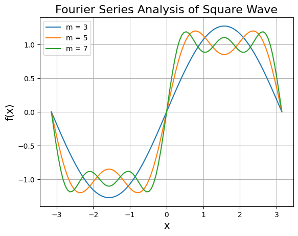
Output:

• Multiple curves showing how the square wave approximation improves as more Fourier terms are added.

import numpy as np
import matplotlib.pyplot as plt

k = 1
pi = np.pi

for m in range(3, 9, 2):
    xrange = np.linspace(-pi, pi, 100);xrange
    n = np.arange(1, m, 2)[:, np.newaxis];n

    fsum = (4*k/pi)*np.sum(np.sin(xrange*n)/n, axis=0)
    plt.plot(xrange, fsum, label = f"m = {m}")
plt.xlabel("x", fontsize =14)
plt.ylabel("f(x)", fontsize =14)
plt.title("Fourier Series Analysis of Square Wave", fontsize = 16)
plt.legend()
plt.grid()
plt.show()

import numpy as np
import matplotlib.pyplot as plt

k = 1
pi = np.pi
xrange = np.linspace(-pi, pi, 100)

# Create an array for m values (3, 5, 7)
m_values = np.arange(3, 9, 2)[:, np.newaxis]  # Shape (3,1) for broadcasting

# Create an array for n values for each m
n_values = [np.arange(1, m, 2)[:, np.newaxis] for m in m_values.flatten()]

# Compute fsum for all m_values at once
fsum_list = [(4 * k / pi) * np.sum(np.sin(xrange * n) / n, axis=0) for n in n_values]

# Plot all the curves at once
for fsum in fsum_list:
    plt.plot(xrange, fsum, label = f"m = {m}")

plt.xlabel("x", fontsize =14)
plt.ylabel("f(x)", fontsize =14)
plt.title("Fourier Series Analysis of Square Wave", fontsize = 16)
plt.legend()
plt.grid()
plt.show()