Computer Lab Semester - 5

Problem - 1

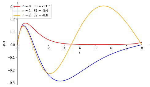
Solve the s-wave Schrödinger equation for the ground state and the first excited state of the hydrogen atom \begin{align} &\frac{d^2u}{dr^2}=A(r)u(r),\\ &A(r) = \frac{2m}{\hbar^2}[V(r)-E],\\ \mbox{where, } &V(r)=-\frac{e^2}{r} \end{align} where, m is the reduced mass of the electron. Obtain the energy eigenvalues and plot the corresponding wave functions. Remember that the ground state energy of the hydrogen atom is ≈-13.6 eV. Take e=3.795 (eVÅ), ħc= 1973(eVÅ) and m=0.511×10\(^6\) eV/c\(^2\).

Time independent Scrodinger equation

\begin{equation} \frac{d^2\psi(x)}{dx^2} + k^2(x)\psi(x) = 0 \end{equation} where, \begin{equation} k^2(x)=\frac{2m}{\hbar^2}(E-V(x)) \end{equation}

We split the second order differential equation into two first order equations as below - \begin{equation} \begin{aligned} &\frac{d\psi}{dx}=\phi(x)\\ &\frac{d\phi}{dx}=-k^2(x)\psi(x) \end{aligned} \end{equation}

import numpy as np
import matplotlib.pyplot as plt
from scipy.integrate import odeint
from scipy.optimize import bisect

# Basic parameters
E0   = -13.6     # approximate ground state energy
e    = 3.795      # charge of electron in eVA
hbarc = 1973   # in eVA
m    = 0.511e6    # in eV/c^2

# Based on the given parameters, calculate 2m/hbar^2c
C  = 2*m/hbarc**2

# Defining Helper Functions

def V(r):
    return - e**2/r

def A(r):
    return C*(V(r)-E)

def dzdr(z, r):
    x, y = z
    dxdr = y
    dydr = A(r)*x
    dzdr = np.array([dxdr, dydr])
    return dzdr

def waveFunc(energy):
    global sol
    global E
    E = energy
    sol = odeint(dzdr, z[0], r)
    return sol[-1, 0]

# setting arrays for storing values

r = np.arange(1e-15, 8, 0.01)
z = np.zeros([len(r),2])
x0 = 0.001
y0 = 1
z[0] = [x0, y0]

# Finding energy eigen values

Energy = np.linspace(-20, 0, 100)
waveFuncRight = np.array([waveFunc(Eval) for Eval in Energy])
sign = np.sign(waveFuncRight)
eigenValue = []
for i in range(len(sign)-1):
    if sign[i] == - sign[i+1]:
        en = bisect(waveFunc, Energy[i], Energy[i+1])
        en = round(en,4)
        eigenValue += [en]

print('Energy Eigen Values are \n'+str(eigenValue))

Energy Eigen Values are
[-13.7319, -3.4059, -0.7694]

# Plotting wavefunctions

def plot():
    fig, ax = plt.subplots(figsize=(8, 5))
    # set the x-spine
    ax.spines['left'].set_position('zero')

    # turn off the right spine/ticks
    ax.spines['right'].set_color('none')
    ax.yaxis.tick_left()

    # set the y-spine
    ax.spines['bottom'].set_position('zero')

    # turn off the top spine/ticks
    ax.spines['top'].set_color('none')
    ax.xaxis.tick_bottom()

plot()

color = ['red', 'blue', 'orange']
for i in range(len(eigenValue)):
    waveFunc(eigenValue[i])
    plt.plot(r, sol[:,0], color=color[i], label='n = '+str(i)+'   E'+str(i)+' = '+str(round(eigenValue[i],1)))

plt.xlabel('r')
plt.ylabel('$\psi(r)$')
plt.legend()
#plt.grid()
plt.show()

Problem - 2

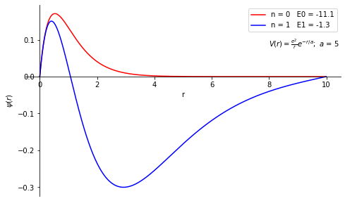
Solve the s-wave radial Schrödinger equation for an atom \begin{align} &\frac{d^2y}{dr^2}=A(r)u(r),\\ &A(r) = \frac{2m}{\hbar^2}[V(r)-E],\\ \mbox{where, } &V(r)=-\frac{e^2}{r} \end{align} Where m is the reduced mass of the system (which can be chosen to be the mass of an electron), for the screened Coulomb potential \begin{align} V(r) = -\frac{e^2}{r}e^{-r/a} \end{align} Find the energy (in eV) of the ground state of the atom to an accuracy of three significant digits. Also, plot the corresponding wave function. Take e=3.795 (eVÅ), and a=3 Å, 5 Å, and 7 Å in the units of ħc = 1973(eVÅ) and m=0.511×10\(^6\) eV/c\(^2\). The ground state energy is expected to be above -12 eV in all three cases.

import numpy as np
import matplotlib.pyplot as plt
from scipy.integrate import odeint
from scipy.optimize import bisect

# Basic parameters
E0 = -12       # approximate ground state energy
e = 3.795      # charge of electron in eVA
hbarc = 1973   # in eVA
m = 0.511e6    # in eV/c^2
a = 5          # in units of angstrum

# Based on the given parameters, calculate 2m/hbar^2c
C = 2*m/hbarc**2

# Defining Helper Functions

def V(r):
    return - (e**2/r )*np.exp(-r/a)

def A(r):
    return C*(V(r)-E)

def dzdr(z, r):
    x, y = z
    dxdr = y
    dydr = A(r)*x
    dzdr = np.array([dxdr, dydr])
    return dzdr

def waveFunc(energy):
    global sol
    global E
    E = energy
    sol = odeint(dzdr, z[0], r)
    return sol[-1, 0]

# setting arrays for storing values

r = np.arange(1e-15, 10, 0.01)
z = np.zeros([len(r),2])
x0 = 0.001
y0 = 1
z[0] = [x0, y0]

# Finding energy eigen values

Energy = np.linspace(-20, 0, 100)
waveFuncRight = np.array([waveFunc(Eval) for Eval in Energy])
sign = np.sign(waveFuncRight)
eigenValue = []
for i in range(len(sign)-1):
    if sign[i] == - sign[i+1]:
        en = bisect(waveFunc, Energy[i], Energy[i+1])
        eigenValue += [en]

print('Energy Eigen Values are \n'+str(eigenValue))

Energy Eigen Values are
[-11.06410939502324, -1.284295766697573]

# Plotting wavefunctions

def plot():
    fig, ax = plt.subplots(figsize=(8, 5))
    # set the x-spine
    ax.spines['left'].set_position('zero')

    # turn off the right spine/ticks
    ax.spines['right'].set_color('none')
    ax.yaxis.tick_left()

    # set the y-spine
    ax.spines['bottom'].set_position('zero')

    # turn off the top spine/ticks
    ax.spines['top'].set_color('none')
    ax.xaxis.tick_bottom()

plot()

color = ['red', 'blue', 'orange']
for i in range(len(eigenValue)):
    waveFunc(eigenValue[i])
    plt.plot(r, sol[:,0], color=color[i], label='n = '+str(i)+'   E'+str(i)+' = '+str(round(eigenValue[i],1)))

plt.xlabel('r')
plt.ylabel('$\psi(r)$')
plt.text(8,0.08, '$V(r)=\\frac{e^2}{r}e^{-r/a};  \\ a$ = '+str(a))
plt.legend()
#plt.grid()
plt.show()

Problem 3

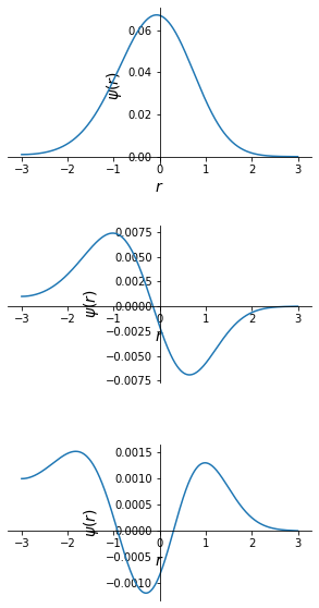
Solve the s-wave Schrodinger equation for the ground state and the first excited state of the hydrogen atom \begin{equation} \frac{d^2y}{dr^2}=A(r)u(r),\hspace{1cm}A(r)=\frac{2m}{\hbar^2}[V(r) - E]\mbox{~where~}V(r)=-\frac{e^2}{r} \end{equation} The anharmonic potential \begin{equation} V(r)=\frac{1}{2}kr^2 + \frac{1}{3}br^3 \end{equation} for the ground state energy (in MeV) of particle to an accuracy of three significant digits. Also, plot the corressponding wave function. Choose \(m=940 MeV/c^2\), \(k=100 MeVfm^{-2}\), \(b=0,10,30 MeVfm^{-3}\). In these units, \(c\hbar=940 MeV/c^2\), \(k=100 MeVfm^{-3}\) for all three cases. The ground state energy is expected to lie in between 90 and 110 MeV for all three cases.

import numpy as np
import matplotlib.pyplot as plt
from scipy.integrate import odeint
from scipy.optimize import newton, bisect, brentq
from scipy.constants import hbar, m_e

# Defining helper functions

# (1) Potential function

def V(r):
    V = (1/2)*k*r**2 + (1/3)*b*r**3
    return V

# (2) Defining A(r)

def A(r):
    a = (2*m_e/ħc**2)*(V(r) - E)
    return a

# (3) Defining Derivative functions of 'y'

def deriv(y, r):
    return np.array([y[1], A(r)*y[0]])

# (4) Defining wave function with respect to energy

def waveFunc(energy):
    global E
    global psi
    E = energy
    psi = odeint(deriv, psi0, r)
    return psi[-1, 0]

# (5) Finding zero of the wavefuncton by Shooting method

def zero(x, y):
    energyEigenValue = []
    s = np.sign(y)
    #s = np.array(s, dtype=int)
    for i in range(len(s)-1):
        if s[i] == -s[i+1]:
            zero = bisect(waveFunc, x[i], x[i+1])
            energyEigenValue.append(zero)
    return energyEigenValue

# Vectorizing the functions
V        = np.vectorize(V)
waveFunc = np.vectorize(waveFunc)
zero = np.vectorize(zero)

# Important parameters

m_e = 940
ħc = 197.3
k = 100
# Initialisation

N = 1000                              # Number of points on x-axis
psi = np.zeros([N, 2])                # To store wave function values and its derivative
psi0 = np.array([0.001, 0])           # wavefunction of initial staes

b = 30
r = np.linspace(-3, 3, N)              # x - axis

En = np.arange(0, 150, 1)
psiRight = waveFunc(En)
#psiRight

def zero(x, psi):
    energyEigenValue = []
    s = np.sign(psi)
    #s = np.array(s, dtype=int)
    for i in range(len(s)-1):
        if s[i] == -s[i+1]:
            zero = bisect(waveFunc, x[i], x[i+1])
            energyEigenValue.append(zero)
    return energyEigenValue

EigenValue = np.array(zero(En, psiRight))
EigenValue

array([ 31.55704024,  92.01776957, 144.81662013])

fig = plt.figure(figsize=(5, 10))
fig.subplots_adjust(hspace=0.4, wspace=0.4)
j=1
for i in range(len(EigenValue)):
    ax = fig.add_subplot(len(EigenValue), 1, j)
    waveFunc(EigenValue[i])
    plt.plot(r, psi.transpose()[0])
    ax.spines['left'].set_position('zero')
    ax.spines['right'].set_color('none')
    ax.spines['top'].set_color('none')
    ax.spines['bottom'].set_position('zero')
    #plt.legend()
    plt.xlabel('$r$', fontsize=14)
    plt.ylabel('$\psi(r)$', fontsize=14)
    j+=1
plt.show()

Problem 4

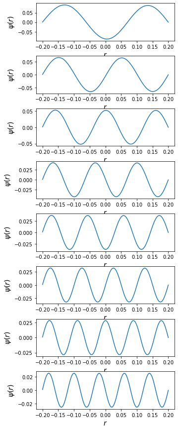
Solve the s-wave Schrodinger equation for the hydrogen molecule \begin{equation} \frac{d^2y}{dr^2}=A(r)u(r),\hspace{1cm}A(r)=\frac{2\mu}{\hbar^2}[V(r) - E] \end{equation} where, \(\mu\) is the reduced mass of the two-atom system for the Morse potential. \begin{equation} V(r)=D\left(e^{-2\alpha r^{\prime}} - e^{-\alpha r^{\prime}}\right),\hspace{0.5cm}r^{\prime}=\frac{r - r_0}{r} \end{equation} Find the lowest vibrational energy (in MeV) of the molecule to an accuracy of three significant digits. Also plot the corressponding wave function. Take \(m=940\times 10^6 eV/c^2\), \(D=0.755501\), \(\alpha=1.44\) and \(r_0=0.131349 \overset{\circ}{A}\)

Morse potential expression given is wrong. The correct form is \begin{align} V(r) &= D \left[1 - e^{-\alpha(r-r_0)}\right]^2\\ V(r) &=D\left(1 - 2e^{-\alpha r^{\prime}} + e^{-2\alpha r^{\prime}}\right), \hspace{0.5cm} r^{\prime}=\frac{r - r_0}{r} \end{align}

import numpy as np
import matplotlib.pyplot as plt
from scipy.integrate import odeint
from scipy.optimize import newton, bisect, brentq
from scipy.constants import hbar, m_e

# Defining helper functions

# (1) Potential function

def V(r, r0, α, D):
    V = D*(1 - np.exp(-α*(r - r0)))**2
    return V

# (2) Defining A(r)

def A(r):
    a = (2*μ/ħc**2)*(V(r, r0, α, D) - E)
    return a

# (3) Defining Derivative functions of 'y'

def deriv(y, r):
    return np.array([y[1], A(r)*y[0]])

# (4) Defining wave function with respect to energy

def waveFunc(energy):
    global E
    global psi
    E = energy
    psi = odeint(deriv, psi0, r)
    return psi[-1, 0]

# (5) Finding zero of the wavefuncton by Shooting method

def zero(x, y):
    energyEigenValue = []
    s = np.sign(y)
    #s = np.array(s, dtype=int)
    for i in range(len(s)-1):
        if s[i] == -s[i+1]:
            zero = bisect(waveFunc, x[i], x[i+1])
            energyEigenValue.append(zero)
    return energyEigenValue

# Vectorizing the functions
V        = np.vectorize(V)
waveFunc = np.vectorize(waveFunc)
zero = np.vectorize(zero)

# Important parameters

μ = 940e6
D = 0.755501
α = 1.44
r0 = 0.131349
ħc = 1973

# Initialisation

N = 100                              # Number of points on x-axis
psi = np.zeros([N, 2])                # To store wave function values and its derivative
psi0 = np.array([0.001, 2])           # wavefunction of initial staes


r = np.linspace(-0.2, 0.2, 100)              # x - axis

En = np.arange(0, 15, 1)
psiRight = waveFunc(En)
#psiRight

def zero(x, psi):
    energyEigenValue = []
    s = np.sign(psi)
    #s = np.array(s, dtype=int)
    for i in range(len(s)-1):
        if s[i] == -s[i+1]:
            zero = bisect(waveFunc, x[i], x[i+1])
            energyEigenValue.append(zero)
    return energyEigenValue

EigenValue = np.array(zero(En, psiRight))
EigenValue

array([ 1.21457505,  2.10732938,  3.2543345 ,  4.65597459,  6.31235437,
        8.22351125, 10.389463  , 12.81021612])

fig = plt.figure(figsize=(5, 15))
fig.subplots_adjust(hspace=0.4, wspace=0.4)
j=1
for i in range(len(EigenValue)):
    ax = fig.add_subplot(len(EigenValue), 1, j)
    waveFunc(EigenValue[i])
    plt.plot(r, psi.transpose()[0])
    #plt.legend()
    plt.xlabel('$r$', fontsize=14)
    plt.ylabel('$\psi(r)$', fontsize=14)
    j+=1
plt.show()